This is an excerpt from the project I created for a Scientific Initiation Report in the Territorial Planning bachelor’s degree at UFBAC in 2022.
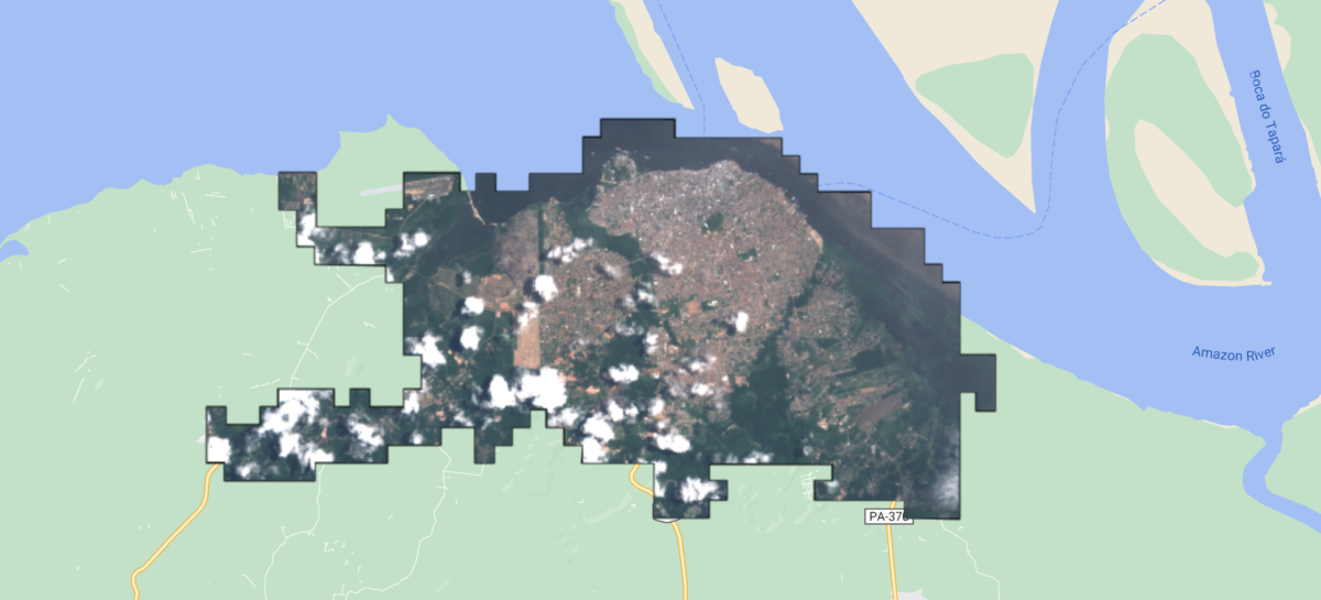
This study performs a temporal analysis of images from the city of Santarém, in Pará 🇧🇷 , covering the period from 2002 to 2022.
The focus is on mapping built-up areas, employing advanced digital image processing techniques and taking into account the cities unique characteristics in the Amazon region.
For the research, one image was used for each year of analysis.
- A LANDSAT 7 image from 2002;
- 9 LANDSAT 5 images referring to time series between 2003 and 2011;
- 8 LANDSAT 8 images referring to time series between 2014 and 2021;
- 7 images from SENTINEL 2 referring to the time series between 2016 and 2022.
Here is an demo of the code used on google earth engine to select this images:
// Define the coordinates of the vertices of the polygon representing the study area
var shapefile = ee.FeatureCollection("projects/santarem-ic/assets/shapefile-santarem");

// Add shapefile to map with default style and center the map
Map.addLayer(shapefile, {}, 'Shapefile');
Map.centerObject(shapefile, 12);

// Dictionary to store image collections by year
var collectionsByYear = {};

// Load LANDSAT images from the collection for each year
for (var year = 2002; year <= 2023; year++) {
  var startDate = year + '-01-01';
  var endDate = year + '-12-31';

  var yearCollection;

  // Which Landsat collection to use for each year range
  if (year === 2002) {
    yearCollection = ee.ImageCollection('LANDSAT/LE07/C01/T1'); // LANDSAT7
  } else if (year >= 2003 && year <= 2011) {
    yearCollection = ee.ImageCollection('LANDSAT/LT05/C01/T1'); // LANDSAT5
  } else {
    yearCollection = ee.ImageCollection('LANDSAT/LC08/C01/T1');
  }

// Apply common filters to the image collection: restrict images to the study area, select images within the specified date range, and sort them chronologically. Then, clip each image to the study area boundaries.

  yearCollection = yearCollection.filterBounds(shapefile)
                                   .filterDate(startDate, endDate)
                                   .sort('system:time_start')
                                   .map(function(image) {
                                     return image.clip(shapefile);
                                   });

  // Store the image collection in the dictionary
  collectionsByYear[year] = yearCollection;
}


// Check the number of images in the collection for a specific year for analysis
// print(collectionsByYear[2022].size())

// Select manually-visual images with the best visibility
var image2021 = ee.Image(collectionsByYear[2021].toList(collectionsByYear[2021].size()).get(2));
var image2020 = ee.Image(collectionsByYear[2020].toList(collectionsByYear[2020].size()).get(2));
// Repeat for other years...

// Array containing all selected images
var bestVisualizations = [
  image2021,
  image2020,
  // Other images here...
];

// Convert the array to an ImageCollection
var imageCollection = ee.ImageCollection.fromImages(bestVisualizations);

// Loop to double-check the Coordinate Reference System of each image
bestVisualizations.forEach(function(image, index) {
  var singleBand = image.select('B4');
  var crs = singleBand.projection().getInfo().crs;
  print("The CRS of the image for the year " + (2002 + index) + " is: ", crs);
});


// EXPORT
// List of years to name the exported images
var years = [
  2002, 2003, 2004, 2005, 2006,
  2007, 2008, 2009, 2010, 2011,
  2014, 2015, 2016,
  2017, 2018, 2019, 2020, 2021
];

// Export images to Google Drive
var imagesToExport = imageCollection.toList(imageCollection.size());

var size = imagesToExport.size().getInfo();

for (var i = 0; i < size; i++) {
  var image = ee.Image(imagesToExport.get(i));

  // Convert all bands to UInt16 to ensure compatibility
  image = image.toUint16();

  // Get the corresponding year to name the image
  var year = years[i];

  // Export the image to Google Drive
  Export.image.toDrive({
    image: image,
    description: 'Image_' + year,
    scale: 30,
    region: shapefile.geometry(),
    fileFormat: 'GeoTIFF'
  });
}
As can be seen in Figure 6, Landsat 8 images have a lower spatial resolution, are more pixelated, and are sufficient to evaluate the distribution and direction of urban sprawl, mainly because the LANDSAT mission is much older and much older than SENTINEL, being essential for time series.
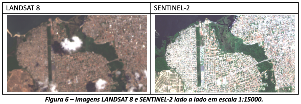
On the other hand, Sentinel 2 images, with their higher spatial resolution, are more appropriate for intra-urban identification and analysis, such as for analyzing densification within the urban area, it is also more assertive for differentiating different types of vegetation and identifying areas of exposed soil.
Therefore, when classifying the LANDSAT images, this work chose to use only 3 classes and in the SENTINEl images, 5 classes.
Initially, it was decided to use the Landsat 7 image series, however, during the course of the study, it was discovered that the Enhanced Thematic Mapper Plus (ETM+) sensor, the mission’s main sensor, broke in 2003. With this failure , the images began to present data gaps, as can be seen in Figure 7, compromising their usefulness for the analyzes presented here.
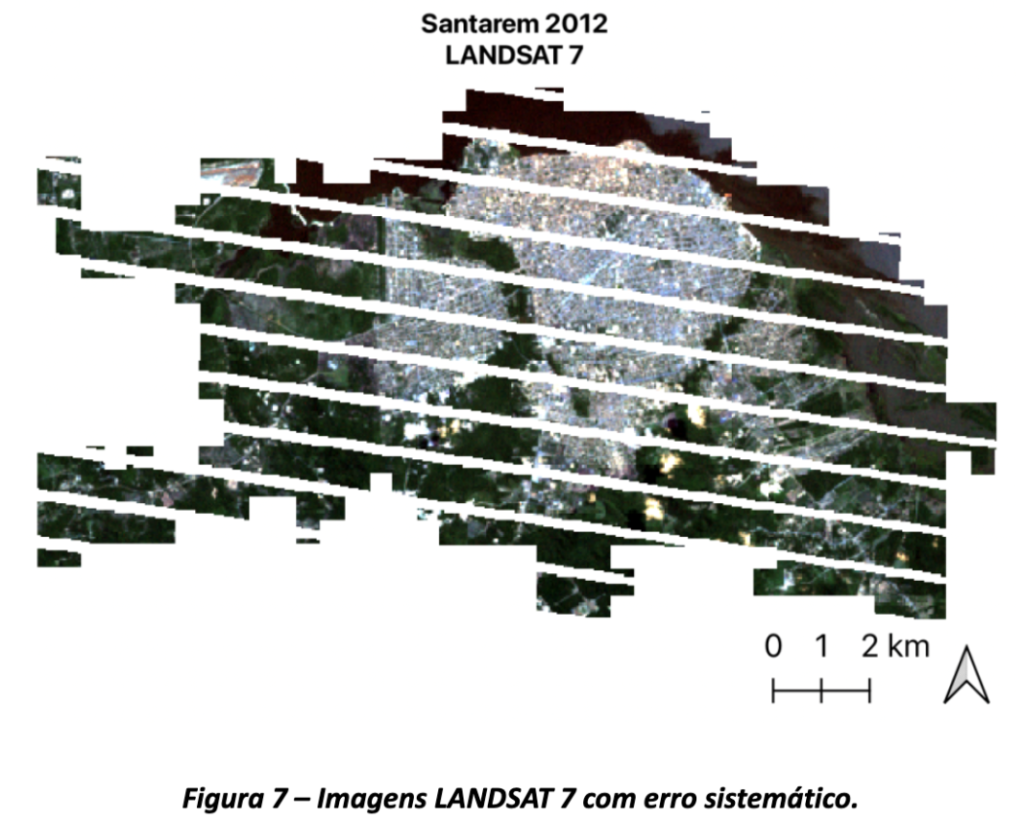
Given this limitation, only one image from LANDSAT 7 was used for the year 2002 and, in the period from 2003 to 2011, images from LANDSAT 5 were used.
No images were used for 2012 and 2013 because they were mostly cloudy and, from 2014 onwards until 2021, images from LANDSAT 8 were used.
Both Landsat 5 and 7 have the same spatial resolution of 30 meters in the visible and infrared bands, with small differences in the spectral range of some bands, which allows this exchange without major loses.
For collection, manipulation and analysis, the following software and techniques were used:
- Google Earth Engine platform for pre-processing satellite images and unsupervised classification, using JavaScript language, using the Random Forest algorithm – (checkout the GitHub repo here);
- Google Colab platform and Python language for analyzing generated classifications;
- QGIS 3.28 for producing thematic maps.
Furthermore, the Random Forest machine learning algorithm was used to manually categorize the images, according to criteria relevant to the region under study. This process was complemented with texture metrics, as indicated in the specialized literature.
Results and discussion of results
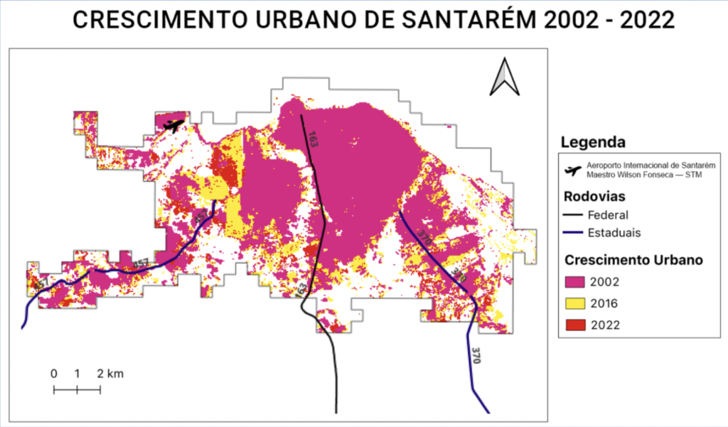
The results are in line with the conclusions of the literature, which indicate that Amazonian cities have recently grown towards the road typology pattern more than the old growth pattern based on the waterway logic.
The literature also points to cities in which the typology is hybrid, as in the case of Santarém, which still continues to grow close to the coastal strip. On the comparison below between Landsat images from 2002 and 2022, it is possible to verify the expansion of the built area.

The city of Santarém grew especially in the regions adjacent to the Fernando Guilhon Highway, where the PA-457 state highway ends and around the roads that extend east towards the airport (figure below).
In addition, there are expansions along the state highways Santarém Curua-Una (PA-370) and Rodovia Everaldo Martins (PA-457), as well as along the federal highway 163, which leads to the edge of the city, where urbanization was already underway. well consolidated in 2002, the beginning of the time series analyzed.
The classification proposed by Gonçalves et al. (2021) proves to be the most accurate approach when dealing with Amazonian cities since it defines the “Built Area” class not only as impermeable surfaces, but also other elements that demonstrate human activities such as internal spaces of lots and roads with exposed soil.